How to use MLFlow with TensorFlow?

Overfitting causes serious headaches when training ML/DL models. But in this article, you’ll see how just a few lines of code can generate data augmentations and boost your model’s performance on the validation set. Additionally, you’ll learn how to properly measure the effect of data augmentation using MLflow’s experiment tracking.

To accomplish the above, we’ll walk you through:

1. Creating a simple Deep Learning model for image detection with tf.keras

2. Adding a few lines for data augmentation support

3. Setting up experiment tracking with MLflow and checking whether our augmentation helps reduce overfitting

What is Data Augmentation?

When creating and training a model, it’s easy to run into all sorts of problems along the way. One common issue is overfitting. Overfitting occurs when a model memorises the training set to a point where it performs worse when being evaluated on data that it has not seen before. Ideally, we want to train a model to learn how you generalize by using training data so it can have the same accuracy on previously unseen data.

What causes overfitting? There are several reasons, the most prevalent being lack of data or not enough regularization used in the network’s architecture. Some techniques can be applied to prevent overfitting, but — especially when it comes to computer vision tasks — there is an easy-to-implement technique that can reduce overfitting: Data Augmentation.

Data augmentation takes a single image and applies random, but realistic, transformations to it. These alterations include changes to the image’s orientation, location, scale, brightness, or combinations of multiple ones.

How can data augmentation reduce overfitting? Because neural networks don’t learn the same way humans do, they can look at different variations of a single image and understand them as unique ones. This gives your model more data to work with.

Data augmentation techniques performed on a single image of a cat

Solving mask detection using TensorFlow

To demonstrate the effect of data augmentation on overfitting, we’ll be using this dataset from Kaggle. It has only 853 images which contain 4072 unique faces. In addition, the dataset comes with annotations which pinpoint the exact coordinate of each face in one image, as well as categorizing them into three classes:

1. with mask

2. without mask

3. mask worn incorrectly

The first step in our script is to create a custom dataset by organising each face into one of three folders corresponding to the aforementioned classes and cropping them into 50 x 50 pixel images, as shown below.

We then split the organised dataset into training and validation subsets, by taking advantage of the Keras image_dataset_from_directory function, which quickly splits and shuffles all data into each subset. In this example, we use 80% for training and 20% for validation and make sure there is no overlap between each subset by giving a unique seed value.

IMG_RESIZE = 50
batch_size = 32
seed = 123
split = 0.2

train_ds = tf.keras.preprocessing.image_dataset_from_directory(
    '/content/dataset/',
    validation_split=split,
    subset='training',
    shuffle=True,
    seed=seed,
    batch_size=batch_size,
    image_size=(IMG_RESIZE, IMG_RESIZE),
)

val_ds = tf.keras.preprocessing.image_dataset_from_directory(
    '/content/dataset/',
    validation_split=split,
    subset='validation',
    shuffle=True,
    seed=seed,
    batch_size=batch_size,
    image_size=(IMG_RESIZE, IMG_RESIZE),
)

We are using a conventional (or should we say convolutional?) approach for our model:

1. A rescaling layer, to standardise RGB channel values into a [0, 1] range

2. Three 2D convolution blocks, each followed by a max pooling layer

3. A dropout regularisation layer, to randomly drop out 20% of the output units

4. A flatten layer, to reshape the tensor into a one-dimensional array

5. Two dense layers, the first one having 128 units activated by a ReLU function and the second one with the final 3 output classes (with mask, without mask, and mask worn incorrectly)

model = Sequential([
  data_augmentation,
  layers.Rescaling(1./255),
  layers.Conv2D(16, 3, padding='same', activation='relu'),
  layers.MaxPooling2D(),
  layers.Conv2D(32, 3, padding='same', activation='relu'),
  layers.MaxPooling2D(),
  layers.Conv2D(64, 3, padding='same', activation='relu'),
  layers.MaxPooling2D(),
  layers.Dropout(0.2),
  layers.Flatten(),
  layers.Dense(128, activation='relu'),
  layers.Dense(len(train_ds.class_names))
]) 

The model is now ready to be compiled and trained.

epochs = 15
optimizer ='adam'
metrics = ['accuracy']

model.compile(optimizer=optimizer,
loss=tf.keras.losses.SparseCategoricalCrossentropy(from_logits=True),
metrics=metrics)

history = model.fit(
  train_ds,
  validation_data=val_ds,
  epochs=epochs
) 

With the trained model, we can now put it to test by classifying images it hasn’t seen before from a different dataset in Kaggle.

The above image shows how the model performed on a random selection from the new dataset. Each image is labelled with the class the model thinks the face being analysed belongs to, as well as the level of certainty the guess is being made with. As we can see, the model is still not perfect, as it only guessed 4 out of 9 correctly.

In the following sections, we will test whether data augmentation improves the model’s performance as we take advantage of MLflow to track the experiments and select the best model.

Tracking experiments with MLflow

Machine learning development can become disorganized very quickly. There many different tools for each phase of the machine learning lifecycle, which in turn make developers dependent on multiple libraries. When experimenting with models, it’s virtually impossible to track and reproduce results.

MLflow presents itself as an open-source platform for the entire machine learning lifecycle. This tool is composed of three main components: Tracking, Projects, and Models; but today we’ll only be focusing on Tracking.

MLflow Tracking provides both an API and a UI that helps visualise metadata about training sessions. For a unique experiment, we can log and store:

1. hyperparameters

2. metrics

3. artifacts

4. source code used to build the model

5. trained model

With a few lines of code, we can compare and view the outputs from multiple training sessions to quickly gain an understanding of which model performed the best.

Comparing and fine-tuning model runs

For a quick setup with Google Colab, let’s use a lightweight managed version of MLflow provided by the Databricks Community. This allows machine learning researchers to run and track their experiments for free.

Run the below commands to start. After installing MLflow and the CLI tool for Databricks, a prompt will appear requesting your Databricks login information.

!pip install mlflow --quiet
!databricks configure --host https://community.cloud.databricks.com/ 

Now that MLflow has access to your Databricks account, configure the URI and the experiment’s location.

mlflow.set_tracking_uri("databricks")
mlflow.set_experiment("/Users/username/experiment") 

You’re are all set to run your training sessions now that Google Colab and MLflow are communicating. Since we are using TensorFlow, tracking your experiment is as easy as running the command mlflow.tensorflow.autolog() before initialising your model. But in the cases you know exactly what you need to log, you can do so manually with the following commands:

mlflow.log_param("num_dimensions", 8)
mlflow.log_metric("accuracy", 0.1)
mlflow.log_artifact("roc.png") 

Next, let’s compare how data augmentation impacts the our model’s performance. To do so, create a new layer that will be placed right at the beginning of our model. Our new layer performs random horizontal flips, rotations, and zooms.

data_augmentation = keras.Sequential(
  [
    layers.RandomFlip("horizontal",
                      input_shape=(IMG_RESIZE,
                                  IMG_RESIZE,
                                  3)),
    layers.RandomRotation(0.1),
    layers.RandomZoom(0.1),
  ]
) 

Transformations made by the data augmentation layer in our dataset

The data augmentation layer’s impact is obvious, as you can see below. Out of the nine faces, the model only made one incorrect guess.

Heading over to the MLflow interface, you can see a rundown of all the training sessions you made.

When selecting a specific run, you can get access to all artifacts produced by the run. This includes the trained model that can be loaded directly from MLflow after a training session is finished.

In the rundown, you can select two different runs and compare the results with and without data augmentation. When comparing the two runs, and after plotting the accuracy and loss values for the training and validation sets using MLflow’s built-in scatter plot, you’ll see the following graphs:

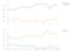
Without data augmentation

With data augmentation

While analysing the first run without data augmentation, both values for accuracy and loss are off by large margins. The difference between training and validation is a clear sign of overfitting. The second run with data augmentation performed a lot better and the difference between values is minimal.

By analysing the values and plots on MLflow, it is clear that data augmentation indeed made an impact on the original model, resulting in better results and more accurate predictions.

You can play with the code developed for this experiment in Google Colab notebooks here.